Transport across sections

mom6_tools.section_transports collection of functions for computing and plotting time-series of transports across pre-defined vertical sections.

The goal of this notebook is the following:

server as an example on how to post-process the CESM/MOM6 vertical sections defined in diag_table. The location of the current vertical sections computed online can be found at the end of this notebook;
evaluate model experiments by comparing transports against observed estimates;

[1]:

%load_ext autoreload
%autoreload 2

[2]:

%matplotlib inline
import warnings
warnings.filterwarnings("ignore")
from mom6_tools.section_transports import Transport, options
import matplotlib.pyplot as plt
from mom6_tools.m6toolbox import cime_xmlquery
import xarray as xr
import yaml, os, numpy

[3]:

# Read in the yaml file
diag_config_yml_path = "diag_config.yml"
diag_config_yml = yaml.load(open(diag_config_yml_path,'r'), Loader=yaml.Loader)

[4]:

# create an empty class object
class args:
    pass

[5]:

caseroot = diag_config_yml['Case']['CASEROOT']
args.casename = cime_xmlquery(caseroot, 'CASE')
DOUT_S = cime_xmlquery(caseroot, 'DOUT_S')
if DOUT_S:
  OUTDIR = cime_xmlquery(caseroot, 'DOUT_S_ROOT')+'/ocn/hist/'
else:
  OUTDIR = cime_xmlquery(caseroot, 'RUNDIR')

print('Output directory is:', OUTDIR)
print('Casename is:', args.casename)

Output directory is: /glade/derecho/scratch/gmarques/archive/g.e30_a03c.GJRAv4.TL319_t232_wgx3_hycom1_N75.2024.079/ocn/hist/
Casename is: g.e30_a03c.GJRAv4.TL319_t232_wgx3_hycom1_N75.2024.079

[6]:

# load sections where transports are computed online
sections = diag_config_yml['Transports']['sections']

Define the arguments expected by class “Transport”. These have been hard-coded here fow now…

[7]:

args.infile = OUTDIR
# set avg dates
avg = diag_config_yml['Avg']
args.start_date = '0001-01-01' # override start date
args.end_date = avg['end_date']
args.label = ''
args.parallel = False
args.debug = False

Observed flows, more options can be added here

Griffies et al., 2016: OMIP contribution to CMIP6: experimental and diagnostic protocol for the physical component of the Ocean Model Intercomparison Project. Geosci. Model. Dev., 9, 3231-3296. doi:10.5194/gmd-9-3231-2016

Below we define a function for plotting transport time series. Note the following:

green = mean transport is within observed values

red = mean transport is not within observed values

gray = either there isn’t observed values to compare with or just a mean value is available (not a range)

[8]:

def plotPanel(section,observedFlows=None,colorCode=True):
    plt.figure(figsize=(7,3))
    ax = plt.subplot(1,1,1,)
    color = '#c3c3c3'; obsLabel = None
    if section.label in observedFlows.keys():
      if isinstance(observedFlows[section.label][1:],list) and isinstance(observedFlows[section.label][1:][0],float):
        if colorCode == True:
          if min(observedFlows[section.label][1:]) <= section.data.mean() <= max(observedFlows[section.label][1:]):
            color = '#90ee90'
          else: color = '#f26161';
        obsLabel = str(min(observedFlows[section.label][1:])) + ' to ' + str(max(observedFlows[section.label][1:]))
      else: obsLabel = str(observedFlows[section.label][1:]);
    plt.plot(section.time,section.data,color=color)
    plt.title(section.label,fontsize=14)
    plt.text(0.04,0.11,'Mean = '+'{0:.2f}'.format(section.data.mean()),transform=ax.transAxes,fontsize=14)
    if obsLabel is not None: plt.text(0.04,0.04,'Obs. = '+obsLabel,transform=ax.transAxes,fontsize=14)
    if section.ylim is not None: plt.ylim(section.ylim)
    plt.ylabel('Transport (Sv)',fontsize=14); plt.xlabel('Time since beginning of run (yr)',fontsize=14)
    plt.grid()
    return

Plot section transports in alphabetical order

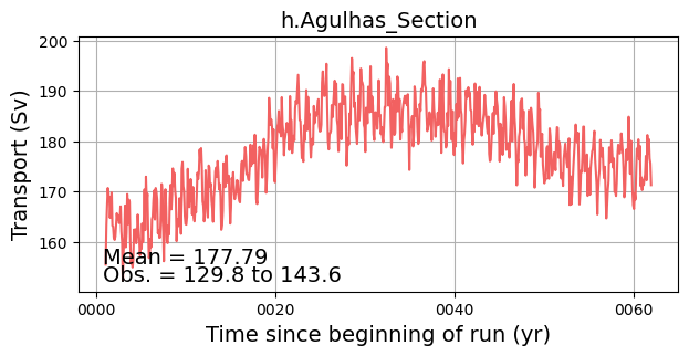
Agulhas Section

[9]:

ds = []
agulhas = Transport(args,sections,'h.Agulhas_Section',debug=False); ds.append(agulhas)
plotPanel(agulhas, observedFlows=sections)

ERROR 1: PROJ: proj_create_from_database: Open of /glade/work/gmarques/conda-envs/mom6-tools/share/proj failed

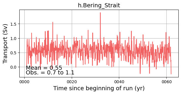
../_images/examples_section_transports_14_1.png

Bering Strait

[10]:

bering = Transport(args, sections, 'h.Bering_Strait'); ds.append(bering)
plotPanel(bering, observedFlows=sections)

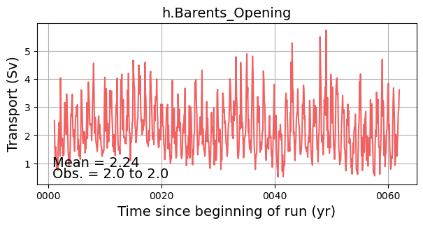
../_images/examples_section_transports_16_0.png

Barents opening

[11]:

barents = Transport(args, sections, 'h.Barents_Opening'); ds.append(barents)
plotPanel(barents, observedFlows=sections)

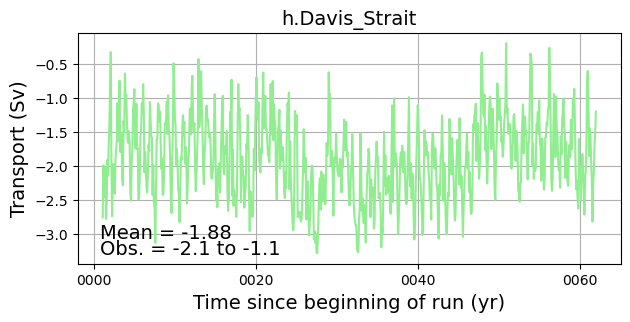
../_images/examples_section_transports_18_0.png

Davis Strait

[12]:

davis = Transport(args, sections,'h.Davis_Strait'); ds.append(davis)
plotPanel(davis, observedFlows=sections)

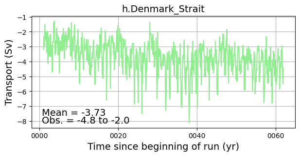
../_images/examples_section_transports_20_0.png

Denmark Strait

[13]:

denmark = Transport(args, sections,'h.Denmark_Strait'); ds.append(denmark)
plotPanel(denmark, observedFlows=sections)

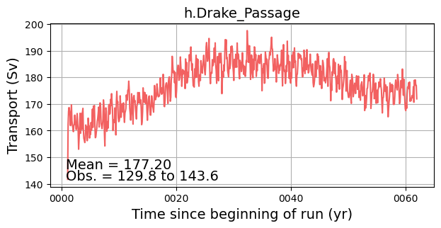
../_images/examples_section_transports_22_0.png

Drake Passage

[14]:

drake = Transport(args, sections,'h.Drake_Passage'); ds.append(drake)
plotPanel(drake, observedFlows=sections)

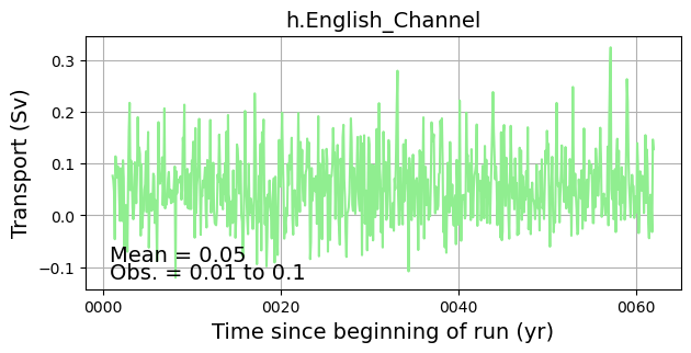
../_images/examples_section_transports_24_0.png

English Channel

[15]:

english = Transport(args, sections, 'h.English_Channel'); ds.append(english)
plotPanel(english, observedFlows=sections)

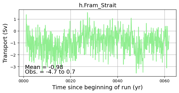
../_images/examples_section_transports_26_0.png

Fram Strait

[16]:

fram = Transport(args, sections, 'h.Fram_Strait'); ds.append(fram)
plotPanel(fram, observedFlows=sections)

../_images/examples_section_transports_28_0.png

Florida Bahamas

[17]:

#florida1 = Transport(args, sections, 'h.Florida_Bahamas', debug=True); ds.append(florida1)
#plotPanel(florida1, observedFlows=sections)

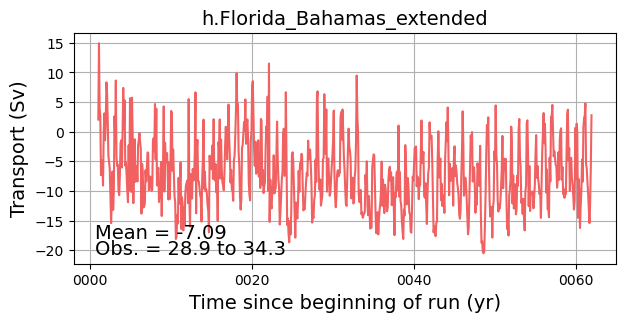
Florida Bahamas extended

[18]:

florida2 = Transport(args, sections, 'h.Florida_Bahamas_extended'); ds.append(florida2)
plotPanel(florida2, observedFlows=sections)

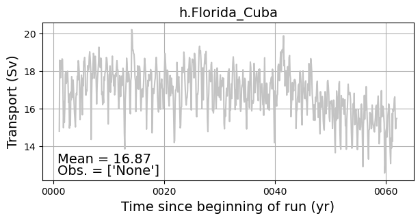
../_images/examples_section_transports_32_0.png

Florida Cuba

[19]:

florida3 = Transport(args, sections, 'h.Florida_Cuba'); ds.append(florida3)
plotPanel(florida3, observedFlows=sections)

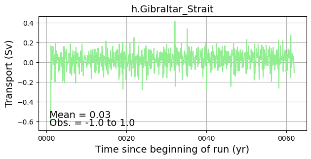
../_images/examples_section_transports_34_0.png

Gibraltar Strait

[20]:

gibraltar = Transport(args, sections, 'h.Gibraltar_Strait'); ds.append(gibraltar)
plotPanel(gibraltar, observedFlows=sections)

../_images/examples_section_transports_36_0.png

Iceland Norway

[21]:

#iceland = Transport(args, sections, 'h.Iceland_Norway', debug=True); ds.append(iceland)
#plotPanel(iceland, observedFlows=sections)

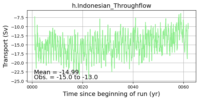
Indonesian Throughflow

[22]:

indo = Transport(args, sections, 'h.Indonesian_Throughflow'); ds.append(indo)
plotPanel(indo, observedFlows=sections)

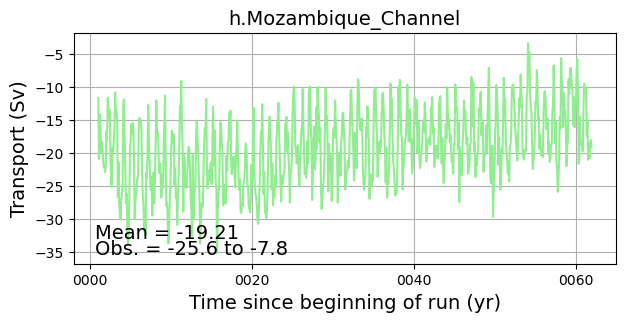
../_images/examples_section_transports_40_0.png

Mozambique Channel

[23]:

mozambique = Transport(args, sections, 'h.Mozambique_Channel'); ds.append(mozambique)
plotPanel(mozambique, observedFlows=sections)

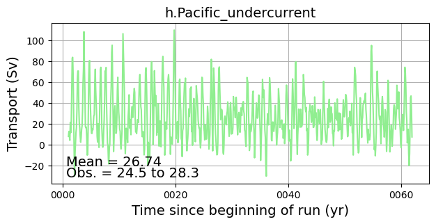
../_images/examples_section_transports_42_0.png

Pacific undercurrent

[24]:

euc = Transport(args, sections, 'h.Pacific_undercurrent'); ds.append(euc)
plotPanel(euc, observedFlows=sections)

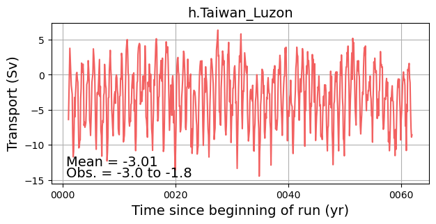
../_images/examples_section_transports_44_0.png

Taiwan Luzon

[25]:

taiwan = Transport(args, sections, 'h.Taiwan_Luzon'); ds.append(taiwan)
plotPanel(taiwan, observedFlows=sections)

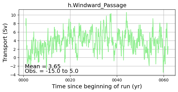
../_images/examples_section_transports_46_0.png

Windward Passage

[26]:

windward = Transport(args, sections, 'h.Windward_Passage'); ds.append(windward)
plotPanel(windward, observedFlows=sections)

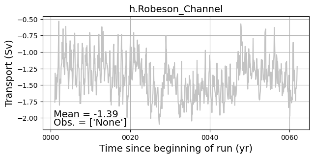
../_images/examples_section_transports_48_0.png

Robeson_Channel

[27]:

roberson = Transport(args, sections, 'h.Robeson_Channel'); ds.append(roberson)
plotPanel(roberson, observedFlows=sections)

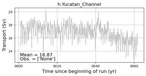
../_images/examples_section_transports_50_0.png

Yucatan_Channel

[28]:

yucatan = Transport(args, sections, 'h.Yucatan_Channel'); ds.append(yucatan)
plotPanel(yucatan, observedFlows=sections)

../_images/examples_section_transports_52_0.png

Bosporus_Strait

[31]:

#bosporus = Transport(args, sections, 'h.Bosporus_Strait', debug=True); ds.append(bosporus)
#plotPanel(bosporus, observedFlows=sections)

Save netcdf

[34]:

print('Saving netCDF file with transports...\n')
if not os.path.isdir('ncfiles'):
      os.system('mkdir -p ncfiles')

# create a dataaray
labels = [];
for n in range(len(ds)): labels.append(ds[n].label)
var = numpy.zeros((len(ds),len(ds[0].time)))
ds_out = xr.Dataset(data_vars={ 'transport' : (('sections', 'time'), var)},
                       coords={'sections': labels,
                               'time': ds[0].time})
for n in range(len(ds)):
  ds_out.transport.values[n,:] = ds[n].data

ds_out.to_netcdf('ncfiles/'+args.casename+'_section_transports.nc')

Saving netCDF file with transports...