Example on how to configure a case using mom6-tools

This is a very simple example showing how to read diag_config.yaml, create a case instance, compute a climatology and visualize the results.

Case Information

• Case:

  • CASEROOT: Path to the root directory of the case: /glade/work/gmarques/cesm.cases/G/g.e30_a03c.GJRAv4.TL319_t232_wgx3_hycom1_N75.2024.079/

  • OCN_DIAG_ROOT: Directory for ocean diagnostics files: ncfiles/

  • SNAME: Identifier or short name of the case: "079"

---

Average Dates

• Avg:

  • start_date: Start date for averaging data: '0031-01-01'

  • end_date: End date for averaging data: '0062-01-01'

---

CESM History File Naming Conventions

• Fnames:

  • rho2: Format for density files: .mom6.h.rho2.????-??.nc

  • z: Format for depth files: .mom6.h.z.????-??.nc

  • native: Format for native files: .mom6.h.native.????-??.nc

  • sfc: Surface files naming convention: .mom6.h.sfc.????-??.nc

  • static: Static files naming convention: .mom6.h.static.nc

  • geom: Ocean geometry files naming convention: .mom6.h.ocean_geometry.nc

---

Transport Sections

• Transports:

  • sections: List of sections where transports are computed, including observational estimates where applicable:

    • ``h.Agulhas_Section``: Uses umo component, range [129.8, 143.6]

    • ``h.Barents_Opening``: Uses vmo component, range [2.0]

    • ``h.Bering_Strait``: Uses vmo component, range [0.7, 1.1]

    • (Additional sections follow similar structure)

---

Ocean Catalog Path

• oce_cat: Path to the ocean-related datasets catalog: /glade/u/home/gmarques/libs/oce-catalogs/reference-datasets.yml

from mom6_tools.m6toolbox import cime_xmlquery
import yaml, os
import numpy as np
import xarray as xr
import matplotlib
from mom6_tools import m6toolbox
import warnings
warnings.filterwarnings('ignore')

# Read in the yaml file
diag_config_yml_path = "diag_config.yml"
diag_config_yml = yaml.load(open(diag_config_yml_path,'r'), Loader=yaml.Loader)

caseroot = diag_config_yml['Case']['CASEROOT']
casename = cime_xmlquery(caseroot, 'CASE')
DOUT_S = cime_xmlquery(caseroot, 'DOUT_S')
if DOUT_S:
  OUTDIR = cime_xmlquery(caseroot, 'DOUT_S_ROOT')+'/ocn/hist/'
else:
  OUTDIR = cime_xmlquery(caseroot, 'RUNDIR')

print('Output directory is:', OUTDIR)

Output directory is: /glade/derecho/scratch/gmarques/archive/g.e30_a03c.GJRAv4.TL319_t232_wgx3_hycom1_N75.2024.079/ocn/hist/

print('Casename is:', casename)

Casename is: g.e30_a03c.GJRAv4.TL319_t232_wgx3_hycom1_N75.2024.079

# create an empty class object
class args:
  pass

args.static = casename+diag_config_yml['Fnames']['static']
args.native = casename+diag_config_yml['Fnames']['native']
args.geom =   casename+diag_config_yml['Fnames']['geom']

# Load the grid
from mom6_tools.MOM6grid import MOM6grid

geom_file = OUTDIR+'/'+args.geom
if os.path.exists(geom_file):
  grd = MOM6grid(OUTDIR+'/'+args.static, geom_file, xrformat=True)
else:
  grd = MOM6grid(OUTDIR+'/'+args.static, xrformat=True)

ERROR 1: PROJ: proj_create_from_database: Open of /glade/work/gmarques/conda-envs/mom6-tools/share/proj failed

MOM6 grid successfully loaded...

# request 6 Dask workers
from ncar_jobqueue import NCARCluster
from dask.distributed import Client

cluster = NCARCluster()
cluster.scale(6)
client = Client(cluster)
client

Client

Client-197af34f-9e18-11ef-a087-3cecef1acc42

Connection method: Cluster object	Cluster type: dask_jobqueue.PBSCluster
Dashboard: https://jupyterhub.hpc.ucar.edu/stable/user/gmarques/High-mem/proxy/8787/status

Launch dashboard in JupyterLab

Cluster Info

PBSCluster

00519662

Dashboard: https://jupyterhub.hpc.ucar.edu/stable/user/gmarques/High-mem/proxy/8787/status	Workers: 0
Total threads: 0	Total memory: 0 B

Scheduler Info

Scheduler

Scheduler-ace8eff9-04d1-437d-935e-857746cff9ed

Comm: tcp://128.117.208.64:37721	Workers: 0
Dashboard: https://jupyterhub.hpc.ucar.edu/stable/user/gmarques/High-mem/proxy/8787/status	Total threads: 0
Started: Just now	Total memory: 0 B

Workers

%time ds = xr.open_mfdataset(OUTDIR+'/'+casename+'.mom6.h.sfc.000?-??.nc', \
         parallel=True, data_vars='minimal', chunks={'time': 12},\
         coords='minimal', compat='override')

CPU times: user 1.44 s, sys: 51.8 ms, total: 1.49 s
Wall time: 27 s

ds

<xarray.Dataset> Size: 41GB
Dimensions:       (time: 3285, yh: 480, xh: 540, xq: 540, yq: 480, nbnd: 2)
Coordinates:
  * xh            (xh) float64 4kB -286.7 -286.0 -285.3 ... 71.33 72.0 72.67
  * yh            (yh) float64 4kB -81.56 -81.46 -81.36 ... 87.65 87.71 87.74
  * time          (time) object 26kB 0001-01-01 12:00:00 ... 0009-12-31 12:00:00
  * nbnd          (nbnd) float64 16B 1.0 2.0
  * xq            (xq) float64 4kB -286.3 -285.7 -285.0 ... 71.67 72.33 73.0
  * yq            (yq) float64 4kB -81.51 -81.41 -81.31 ... 87.68 87.73 87.74
Data variables: (12/16)
    SSH           (time, yh, xh) float32 3GB dask.array<chunksize=(12, 480, 540), meta=np.ndarray>
    tos           (time, yh, xh) float32 3GB dask.array<chunksize=(12, 480, 540), meta=np.ndarray>
    sos           (time, yh, xh) float32 3GB dask.array<chunksize=(12, 480, 540), meta=np.ndarray>
    SSU           (time, yh, xq) float32 3GB dask.array<chunksize=(12, 480, 540), meta=np.ndarray>
    SSV           (time, yq, xh) float32 3GB dask.array<chunksize=(12, 480, 540), meta=np.ndarray>
    mass_wt       (time, yh, xh) float32 3GB dask.array<chunksize=(12, 480, 540), meta=np.ndarray>
    ...            ...
    mlotst        (time, yh, xh) float32 3GB dask.array<chunksize=(12, 480, 540), meta=np.ndarray>
    oml           (time, yh, xh) float32 3GB dask.array<chunksize=(12, 480, 540), meta=np.ndarray>
    average_T1    (time) object 26kB dask.array<chunksize=(12,), meta=np.ndarray>
    average_T2    (time) object 26kB dask.array<chunksize=(12,), meta=np.ndarray>
    average_DT    (time) timedelta64[ns] 26kB dask.array<chunksize=(12,), meta=np.ndarray>
    time_bounds   (time, nbnd) object 53kB dask.array<chunksize=(12, 2), meta=np.ndarray>
Attributes:
    NumFilesInSet:     1
    title:             MOM6 diagnostic fields table for CESM case: g.e30_a03c...
    associated_files:  areacello: g.e30_a03c.GJRAv4.TL319_t232_wgx3_hycom1_N7...
    grid_type:         regular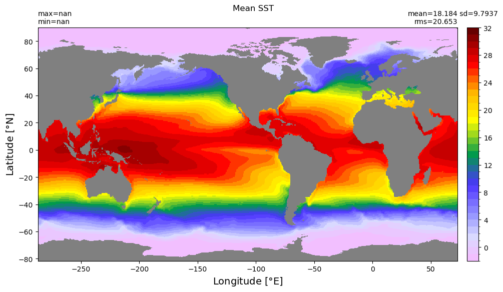
    grid_tile:         N/A

xarray.Dataset

• Dimensions:
  • time: 3285
  • yh: 480
  • xh: 540
  • xq: 540
  • yq: 480
  • nbnd: 2
• Coordinates: (6)
  • xh
    (xh)
    float64
    -286.7 -286.0 -285.3 ... 72.0 72.67

    units :

    degrees_east

    long_name :

    h point nominal longitude

    axis :

    X

    array([-286.666667, -286.      , -285.333333, ...,   71.333333,   72.      ,
             72.666667])

  • yh
    (yh)
    float64
    -81.56 -81.46 ... 87.71 87.74

    units :

    degrees_north

    long_name :

    h point nominal latitude

    axis :

    Y

    array([-81.558125, -81.459689, -81.360114, ...,  87.645456,  87.708781,
            87.740555])

  • time
    (time)
    object
    0001-01-01 12:00:00 ... 0009-12-...

    long_name :

    time

    axis :

    T

    bounds :

    time_bounds

    array([cftime.DatetimeNoLeap(1, 1, 1, 12, 0, 0, 0, has_year_zero=True),
           cftime.DatetimeNoLeap(1, 1, 2, 12, 0, 0, 0, has_year_zero=True),
           cftime.DatetimeNoLeap(1, 1, 3, 12, 0, 0, 0, has_year_zero=True), ...,
           cftime.DatetimeNoLeap(9, 12, 29, 12, 0, 0, 0, has_year_zero=True),
           cftime.DatetimeNoLeap(9, 12, 30, 12, 0, 0, 0, has_year_zero=True),
           cftime.DatetimeNoLeap(9, 12, 31, 12, 0, 0, 0, has_year_zero=True)],
          dtype=object)

  • nbnd
    (nbnd)
    float64
    1.0 2.0

    long_name :

    bounds

    array([1., 2.])

  • xq
    (xq)
    float64
    -286.3 -285.7 -285.0 ... 72.33 73.0

    units :

    degrees_east

    long_name :

    q point nominal longitude

    axis :

    X

    array([-286.333333, -285.666667, -285.      , ...,   71.666667,   72.333333,
             73.      ])

  • yq
    (yq)
    float64
    -81.51 -81.41 ... 87.73 87.74

    units :

    degrees_north

    long_name :

    q point nominal latitude

    axis :

    Y

    array([-81.509049, -81.410045, -81.309895, ...,  87.681   ,  87.728654,
            87.744508])

• Data variables: (16)
  • SSH
    (time, yh, xh)
    float32
    dask.array<chunksize=(12, 480, 540), meta=np.ndarray>

    units :

    m

    long_name :

    Sea Surface Height

    cell_methods :

    area:mean yh:mean xh:mean time: mean

    cell_measures :

    area: areacello

    time_avg_info :

    average_T1,average_T2,average_DT

    Array Chunk Bytes 3.17 GiB 11.87 MiB Shape (3285, 480, 540) (12, 480, 540) Dask graph 324 chunks in 217 graph layers Data type float32 numpy.ndarray

  • tos
    (time, yh, xh)
    float32
    dask.array<chunksize=(12, 480, 540), meta=np.ndarray>

    units :

    degC

    long_name :

    Sea Surface Temperature

    cell_methods :

    area:mean yh:mean xh:mean time: mean

    cell_measures :

    area: areacello

    time_avg_info :

    average_T1,average_T2,average_DT

    standard_name :

    sea_surface_temperature

    Array Chunk Bytes 3.17 GiB 11.87 MiB Shape (3285, 480, 540) (12, 480, 540) Dask graph 324 chunks in 217 graph layers Data type float32 numpy.ndarray

  • sos
    (time, yh, xh)
    float32
    dask.array<chunksize=(12, 480, 540), meta=np.ndarray>

    units :

    psu

    long_name :

    Sea Surface Salinity

    cell_methods :

    area:mean yh:mean xh:mean time: mean

    cell_measures :

    area: areacello

    time_avg_info :

    average_T1,average_T2,average_DT

    standard_name :

    sea_surface_salinity

    Array Chunk Bytes 3.17 GiB 11.87 MiB Shape (3285, 480, 540) (12, 480, 540) Dask graph 324 chunks in 217 graph layers Data type float32 numpy.ndarray

  • SSU
    (time, yh, xq)
    float32
    dask.array<chunksize=(12, 480, 540), meta=np.ndarray>

    units :

    m s-1

    long_name :

    Sea Surface Zonal Velocity

    cell_methods :

    yh:mean xq:point time: mean

    time_avg_info :

    average_T1,average_T2,average_DT

    interp_method :

    none

    Array Chunk Bytes 3.17 GiB 11.87 MiB Shape (3285, 480, 540) (12, 480, 540) Dask graph 324 chunks in 217 graph layers Data type float32 numpy.ndarray

  • SSV
    (time, yq, xh)
    float32
    dask.array<chunksize=(12, 480, 540), meta=np.ndarray>

    units :

    m s-1

    long_name :

    Sea Surface Meridional Velocity

    cell_methods :

    yq:point xh:mean time: mean

    time_avg_info :

    average_T1,average_T2,average_DT

    interp_method :

    none

    Array Chunk Bytes 3.17 GiB 11.87 MiB Shape (3285, 480, 540) (12, 480, 540) Dask graph 324 chunks in 217 graph layers Data type float32 numpy.ndarray

  • mass_wt
    (time, yh, xh)
    float32
    dask.array<chunksize=(12, 480, 540), meta=np.ndarray>

    units :

    kg m-2

    long_name :

    The column mass for calculating mass-weighted average properties

    cell_methods :

    area:mean yh:mean xh:mean time: mean

    cell_measures :

    area: areacello

    time_avg_info :

    average_T1,average_T2,average_DT

    Array Chunk Bytes 3.17 GiB 11.87 MiB Shape (3285, 480, 540) (12, 480, 540) Dask graph 324 chunks in 217 graph layers Data type float32 numpy.ndarray

  • opottempmint
    (time, yh, xh)
    float32
    dask.array<chunksize=(12, 480, 540), meta=np.ndarray>

    units :

    degC kg m-2

    long_name :

    integral_wrt_depth_of_product_of_sea_water_density_and_potential_temperature

    cell_methods :

    area:mean yh:mean xh:mean time: mean

    cell_measures :

    area: areacello

    time_avg_info :

    average_T1,average_T2,average_DT

    standard_name :

    Depth integrated density times potential temperature

    Array Chunk Bytes 3.17 GiB 11.87 MiB Shape (3285, 480, 540) (12, 480, 540) Dask graph 324 chunks in 217 graph layers Data type float32 numpy.ndarray

  • somint
    (time, yh, xh)
    float32
    dask.array<chunksize=(12, 480, 540), meta=np.ndarray>

    units :

    psu kg m-2

    long_name :

    integral_wrt_depth_of_product_of_sea_water_density_and_salinity

    cell_methods :

    area:mean yh:mean xh:mean time: mean

    cell_measures :

    area: areacello

    time_avg_info :

    average_T1,average_T2,average_DT

    standard_name :

    Depth integrated density times salinity

    Array Chunk Bytes 3.17 GiB 11.87 MiB Shape (3285, 480, 540) (12, 480, 540) Dask graph 324 chunks in 217 graph layers Data type float32 numpy.ndarray

  • Rd_dx
    (time, yh, xh)
    float32
    dask.array<chunksize=(12, 480, 540), meta=np.ndarray>

    units :

    m m-1

    long_name :

    Ratio between deformation radius and grid spacing

    cell_methods :

    area:mean yh:mean xh:mean time: mean

    cell_measures :

    area: areacello

    time_avg_info :

    average_T1,average_T2,average_DT

    Array Chunk Bytes 3.17 GiB 11.87 MiB Shape (3285, 480, 540) (12, 480, 540) Dask graph 324 chunks in 217 graph layers Data type float32 numpy.ndarray

  • speed
    (time, yh, xh)
    float32
    dask.array<chunksize=(12, 480, 540), meta=np.ndarray>

    units :

    m s-1

    long_name :

    Sea Surface Speed

    cell_methods :

    area:mean yh:mean xh:mean time: mean

    cell_measures :

    area: areacello

    time_avg_info :

    average_T1,average_T2,average_DT

    Array Chunk Bytes 3.17 GiB 11.87 MiB Shape (3285, 480, 540) (12, 480, 540) Dask graph 324 chunks in 217 graph layers Data type float32 numpy.ndarray

  • mlotst
    (time, yh, xh)
    float32
    dask.array<chunksize=(12, 480, 540), meta=np.ndarray>

    units :

    m

    long_name :

    Ocean Mixed Layer Thickness Defined by Sigma T

    cell_methods :

    area:mean yh:mean xh:mean time: mean

    cell_measures :

    area: areacello

    time_avg_info :

    average_T1,average_T2,average_DT

    standard_name :

    ocean_mixed_layer_thickness_defined_by_sigma_t

    Array Chunk Bytes 3.17 GiB 11.87 MiB Shape (3285, 480, 540) (12, 480, 540) Dask graph 324 chunks in 217 graph layers Data type float32 numpy.ndarray

  • oml
    (time, yh, xh)
    float32
    dask.array<chunksize=(12, 480, 540), meta=np.ndarray>

    units :

    meter

    long_name :

    Thickness of the surface Ocean Boundary Layer calculated by [CVMix] KPP

    cell_methods :

    area:mean yh:mean xh:mean time: mean

    cell_measures :

    area: areacello

    time_avg_info :

    average_T1,average_T2,average_DT

    Array Chunk Bytes 3.17 GiB 11.87 MiB Shape (3285, 480, 540) (12, 480, 540) Dask graph 324 chunks in 217 graph layers Data type float32 numpy.ndarray

  • average_T1
    (time)
    object
    dask.array<chunksize=(12,), meta=np.ndarray>

    long_name :

    Start time for average period

    Array Chunk Bytes 25.66 kiB 96 B Shape (3285,) (12,) Dask graph 324 chunks in 217 graph layers Data type object numpy.ndarray

  • average_T2
    (time)
    object
    dask.array<chunksize=(12,), meta=np.ndarray>

    long_name :

    End time for average period

    Array Chunk Bytes 25.66 kiB 96 B Shape (3285,) (12,) Dask graph 324 chunks in 217 graph layers Data type object numpy.ndarray

  • average_DT
    (time)
    timedelta64[ns]
    dask.array<chunksize=(12,), meta=np.ndarray>

    long_name :

    Length of average period

    Array Chunk Bytes 25.66 kiB 96 B Shape (3285,) (12,) Dask graph 324 chunks in 217 graph layers Data type timedelta64[ns] numpy.ndarray

  • time_bounds
    (time, nbnd)
    object
    dask.array<chunksize=(12, 2), meta=np.ndarray>

    long_name :

    time interval endpoints

    Array Chunk Bytes 51.33 kiB 192 B Shape (3285, 2) (12, 2) Dask graph 324 chunks in 217 graph layers Data type object numpy.ndarray

• Indexes: (6)
  • xh
    PandasIndex

    PandasIndex(Index([-286.66666666666663,              -286.0, -285.33333333333337,
           -284.66666666666663,              -284.0, -283.33333333333326,
           -282.66666666666674,              -282.0, -281.33333333333326,
           -280.66666666666674,
           ...
             66.66666666666652,   67.33333333333326,                68.0,
             68.66666666666652,   69.33333333333326,                70.0,
             70.66666666666652,   71.33333333333326,                72.0,
             72.66666666666674],
          dtype='float64', name='xh', length=540))

  • yh
    PandasIndex

    PandasIndex(Index([-81.55812493176025, -81.45968892243141, -81.36011371758804,
           -81.25938643762682, -81.15749406809196, -81.05442345864881,
           -80.95016132206449, -80.84469423319594,  -80.7380086279867,
           -80.63009080247244,
           ...
            86.50487294857186,  86.72368442615951,  86.92807916262758,
            87.11580151651526,  87.28427233645957,  87.43064950723284,
            87.55197961937547,  87.64545609807651,  87.70878090686321,
            87.74055512340995],
          dtype='float64', name='yh', length=480))

  • time
    PandasIndex

    PandasIndex(CFTimeIndex([0001-01-01 12:00:00, 0001-01-02 12:00:00, 0001-01-03 12:00:00,
                 0001-01-04 12:00:00, 0001-01-05 12:00:00, 0001-01-06 12:00:00,
                 0001-01-07 12:00:00, 0001-01-08 12:00:00, 0001-01-09 12:00:00,
                 0001-01-10 12:00:00,
                 ...
                 0009-12-22 12:00:00, 0009-12-23 12:00:00, 0009-12-24 12:00:00,
                 0009-12-25 12:00:00, 0009-12-26 12:00:00, 0009-12-27 12:00:00,
                 0009-12-28 12:00:00, 0009-12-29 12:00:00, 0009-12-30 12:00:00,
                 0009-12-31 12:00:00],
                dtype='object', length=3285, calendar='noleap', freq='D'))

  • nbnd
    PandasIndex

    PandasIndex(Index([1.0, 2.0], dtype='float64', name='nbnd'))

  • xq
    PandasIndex

    PandasIndex(Index([-286.33333333333337, -285.66666666666663,              -285.0,
           -284.33333333333337, -283.66666666666674,              -283.0,
           -282.33333333333326, -281.66666666666674,              -281.0,
           -280.33333333333326,
           ...
                          67.0,   67.66666666666652,   68.33333333333326,
                          69.0,   69.66666666666652,   70.33333333333326,
                          71.0,   71.66666666666652,   72.33333333333326,
                          73.0],
          dtype='float64', name='xq', length=540))

  • yq
    PandasIndex

    PandasIndex(Index([-81.50904852679943,  -81.4100445212757, -81.30989489722798,
           -81.20858670775536, -81.10610687059054, -81.00244216707667,
           -80.89757924115176,   -80.791504598341, -80.68420460475764,
            -80.5756654861134,
           ...
            86.61595285044066,  86.82781694882009,  87.02417832140226,
            87.20261611085037,   87.3604070055495,  87.49462829656471,
            87.60235982679546,   87.6810004121276,   87.7286543648068,
            87.74450779376627],
          dtype='float64', name='yq', length=480))

• Attributes: (5)

  NumFilesInSet :

  1

  title :

  MOM6 diagnostic fields table for CESM case: g.e30_a03c.GJRAv4.TL319_t232_wgx3_hycom1_N75.2024.079

  associated_files :

  areacello: g.e30_a03c.GJRAv4.TL319_t232_wgx3_hycom1_N75.2024.079.mom6.h.static.nc

  grid_type :

  regular

  grid_tile :

  N/A

%matplotlib inline
# Plot mean SST
from mom6_tools.m6plot import xyplot

area = np.ma.masked_where(grd.wet == 0, np.ma.masked_invalid(grd.areacello))

dummy1 = np.ma.masked_where(grd.wet == 0, ds.tos.mean('time'))

xyplot(dummy1, grd.geolon, grd.geolat, area , suptitle='Mean SST', clim=(-2,32))