Antarctic Intermediate Water (AAIW)
Purpose:
Compute and plot the buoyancy contribution to potential vorticity over the Pacific Sector of the Southern Ocean.
Acknowledgment
This notebook builds on work by John Krasting (NOAA/GFDL). The original version can be found at: https://github.com/jkrasting/mar/blob/main/src/gfdlnb/notebooks/ocean/AAIW_PV.ipynb.
[1]:
%load_ext autoreload
%autoreload 2
[34]:
%matplotlib inline
import warnings
warnings.filterwarnings("ignore")
import matplotlib
import numpy as np
import xarray as xr
import momlevel as ml
from ncar_jobqueue import NCARCluster
from dask.distributed import Client
import cartopy.crs as ccrs
from mom6_tools.MOM6grid import MOM6grid
from mom6_tools.m6toolbox import add_global_attrs
from mom6_tools.m6toolbox import cime_xmlquery
from mom6_tools.m6toolbox import weighted_temporal_mean_vars
from mom6_tools.m6toolbox import geoslice
from mom6_tools.aaiw_pv import plot_aaiw_pv, plot_aaiw_pv_obs
import matplotlib.pyplot as plt
import yaml, os, intake
[3]:
# Read in the yaml file
diag_config_yml_path = "diag_config.yml"
diag_config_yml = yaml.load(open(diag_config_yml_path,'r'), Loader=yaml.Loader)
[4]:
caseroot = diag_config_yml['Case']['CASEROOT']
casename = cime_xmlquery(caseroot, 'CASE')
DOUT_S = cime_xmlquery(caseroot, 'DOUT_S')
if DOUT_S:
  OUTDIR = cime_xmlquery(caseroot, 'DOUT_S_ROOT')+'/ocn/hist/'
else:
  OUTDIR = cime_xmlquery(caseroot, 'RUNDIR')

print('Output directory is:', OUTDIR)
print('Casename is:', casename)
Output directory is: /glade/derecho/scratch/gmarques/archive/g.e30_a03c.GJRAv4.TL319_t232_wgx3_hycom1_N75.2024.079/ocn/hist/
Casename is: g.e30_a03c.GJRAv4.TL319_t232_wgx3_hycom1_N75.2024.079
[5]:
# The following parameters must be set accordingly
######################################################
# add your name and email address below
author = 'Gustavo Marques (gmarques@ucar.edu)'
######################################################
# create an empty class object
class args:
  pass

# load avg dates
avg = diag_config_yml['Avg']

args.infile = OUTDIR
args.monthly = casename+diag_config_yml['Fnames']['z']
args.static = casename+diag_config_yml['Fnames']['static']
args.geom =   casename+diag_config_yml['Fnames']['geom']
args.start_date = avg['start_date']
args.end_date = avg['end_date']
args.casename = casename
args.label = diag_config_yml['Case']['SNAME']
args.savefigs = False
args.outdir = 'PNG/AAIW_PV/'
[6]:
# read grid info
geom_file = OUTDIR+'/'+args.geom
if os.path.exists(geom_file):
  grd = MOM6grid(OUTDIR+'/'+args.static, geom_file, xrformat=True)
else:
  grd = MOM6grid(OUTDIR+'/'+args.static, xrformat=True)

try:
  depth = grd.depth_ocean
except:
  depth = grd.deptho
MOM6 grid successfully loaded...
[7]:
# Coriolis
coriolis = ml.derived.calc_coriolis(grd.geolat)
[8]:
cluster = NCARCluster()
cluster.scale(6)
client = Client(cluster)
client
[8]:
Client
Client-38959a84-e3e2-11ef-a08c-3cecef1b11fa
| Connection method: Cluster object | Cluster type: dask_jobqueue.PBSCluster |
| Dashboard: https://jupyterhub.hpc.ucar.edu/stable/user/gmarques/High-mem/proxy/8787/status |
Cluster Info
PBSCluster
bfe8817c
| Dashboard: https://jupyterhub.hpc.ucar.edu/stable/user/gmarques/High-mem/proxy/8787/status | Workers: 0 |
| Total threads: 0 | Total memory: 0 B |
Scheduler Info
Scheduler
Scheduler-908afe8a-4948-41c8-8958-71cd2f88e652
| Comm: tcp://128.117.208.103:38635 | Workers: 0 |
| Dashboard: https://jupyterhub.hpc.ucar.edu/stable/user/gmarques/High-mem/proxy/8787/status | Total threads: 0 |
| Started: Just now | Total memory: 0 B |
Workers
[9]:
def preprocess(ds):
    ''' Return a dataset desired variables'''
    variables = ['thetao', 'so', 'volcello']
    return ds[variables]
[10]:
print('\n Reading dataset...')
# load data
%time ds = xr.open_mfdataset(OUTDIR+'/'+args.monthly, parallel=True, \
                             combine="nested", concat_dim="time", \
                             preprocess=preprocess).chunk({"time": 12})
 Reading dataset...
CPU times: user 3.3 s, sys: 298 ms, total: 3.6 s
Wall time: 47.2 s
[11]:
print('\n Selecting data between {} and {}...'.format(args.start_date, args.end_date))
%time ds_sel = ds.sel(time=slice(args.start_date, args.end_date))
 Selecting data between 0031-01-01 and 0062-01-01...
CPU times: user 5.1 ms, sys: 179 μs, total: 5.28 ms
Wall time: 5.29 ms
[12]:
attrs =  {
         'description': 'Annual mean thetao, so and volcello',
         'reduction_method': 'annual mean weighted by days in each month',
         'casename': casename
         }
[13]:
ds_ann = weighted_temporal_mean_vars(ds_sel, attrs=attrs)
[14]:
ds_mean = ds_ann.mean("time")
[15]:
%%time
zeta = 0.0
n2 = ml.derived.calc_n2(ds_mean.thetao, ds_mean.so)
pv = ml.derived.calc_pv(zeta, coriolis, n2, interp_n2=False, units="cm")
pv = pv.transpose("z_l", "yh", "xh")
pv = pv.load()
CPU times: user 3.54 s, sys: 292 ms, total: 3.83 s
Wall time: 48 s
[16]:
# Add the latitude and longitude as new coordinates to the pv DataArray
pv = pv.assign_coords({
    "latitude": (("yh", "xh"), grd.geolat.data),
    "longitude": (("yh", "xh"), grd.geolon.data)
})
#pv
[17]:
ds_mean = ds_mean.assign_coords({
    "latitude": (("yh", "xh"), grd.geolat.data),
    "longitude": (("yh", "xh"), grd.geolon.data)
})
#ds_mean
[18]:
#pv['longitude'] = lon
#pv = pv.assign_coords(longitude=lon)
[19]:
pv = geoslice(pv, x=(-180,-70),y=(-65,0), xcoord="longitude", ycoord="latitude")
[20]:
%matplotlib inline
ds_mean.thetao[0,:].plot(vmin=-2, vmax=32)
[20]:
<matplotlib.collections.QuadMesh at 0x147c782d2190>
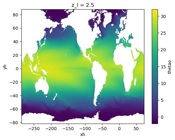
Visulaize selected region
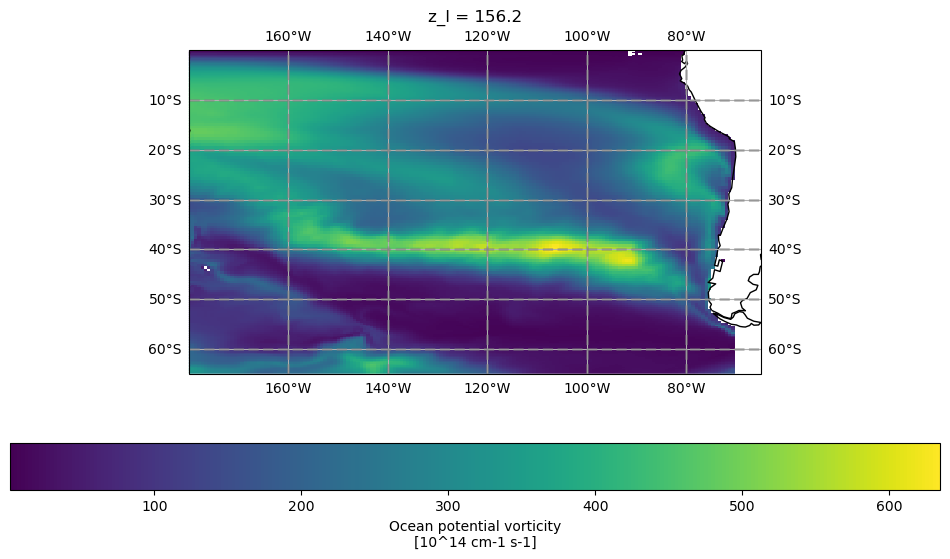
[21]:
fig = plt.figure(figsize=(12, 6))
ax = plt.axes(projection=ccrs.PlateCarree())
ax.coastlines()
ax.gridlines()
pv[8,:].plot(ax=ax, cbar_kwargs={"orientation": "horizontal"}, transform=ccrs.PlateCarree())
ax.gridlines(draw_labels=True, linewidth=2, color='gray', alpha=0.5, linestyle='--')
ax.set_extent([-180, -65, -65, 0], crs=ccrs.PlateCarree())
[22]:
levels, colors = ml.util.get_pv_colormap()
yindex = pv.latitude.mean("xh")
Calcualte the Volume
[23]:
volcello = geoslice(ds_mean.volcello, x=(-180,-70),y=(-65,0),
                             xcoord="longitude", ycoord="latitude")
volume = xr.where(pv > 60.0, volcello, np.nan).sel(z_l=slice(700, None)).sum()
volume = volume.load()
print(f"Volume of water with PV > 60 cm-2 s-1: {float(volume/1.0e15)} x 1.0e^15")
Volume of water with PV > 60 cm-2 s-1: 11.938096092946052 x 1.0e^15
Make zonal mean plots
[24]:
# Take the zonal mean
pv = pv.weighted(grd.areacello.fillna(0)).mean("xh")
[25]:
pv = pv.transpose("z_l", "yh")
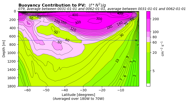
Bouyancy contribution to PV from model
[27]:
%matplotlib inline
args.label = args.label + ', average between ' + args.start_date + ' and ' + args.end_date
plot_aaiw_pv(yindex, pv.z_l, pv, volume, levels, colors, args)
Volume of water with PV > 60 cm-2 s-1: 11.938096092946052 x 1.0e^15
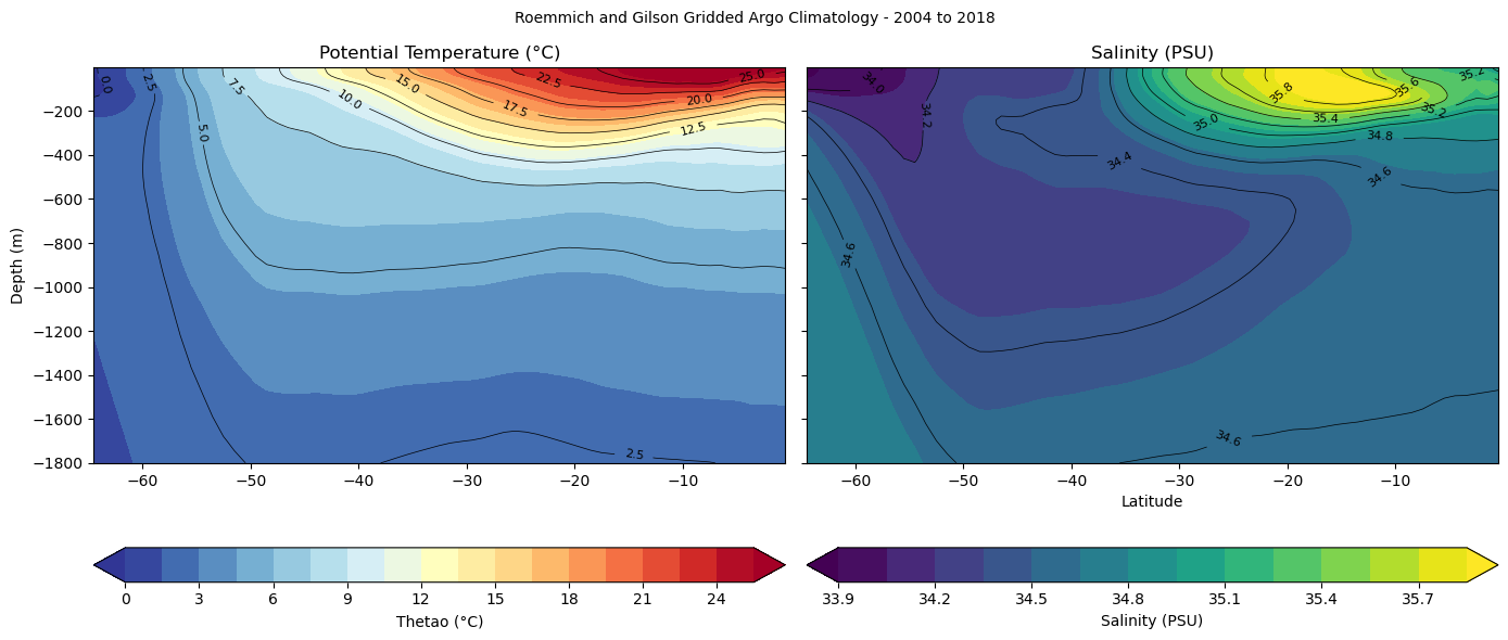
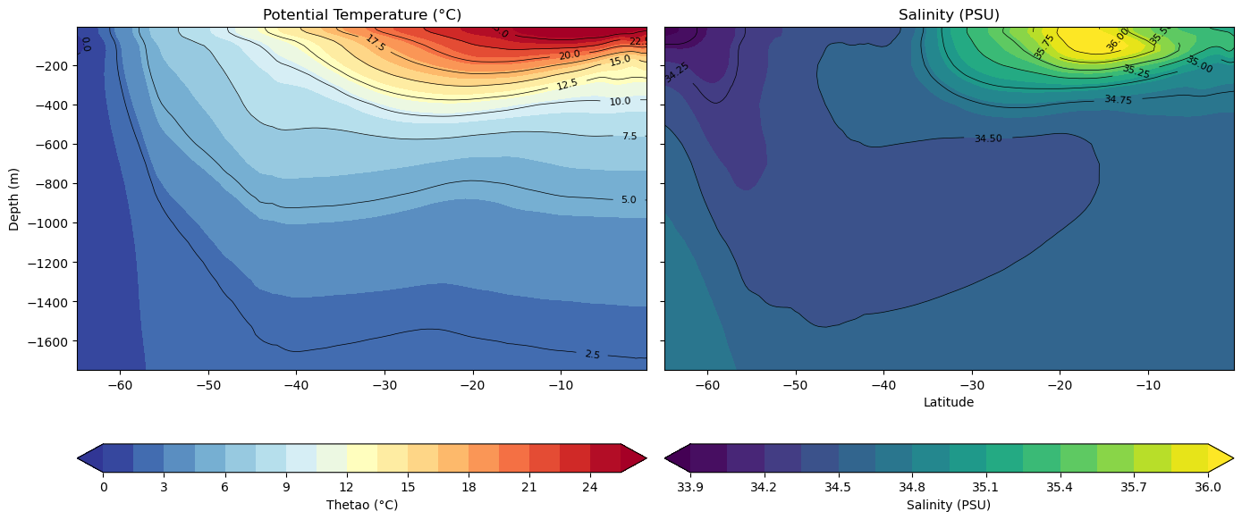
Temperatude and salinity from model
[28]:
thetao = geoslice(ds_mean.thetao, x=(-180,-70),y=(-65,0), xcoord="longitude", ycoord="latitude").weighted(grd.areacello.fillna(0)).mean("xh").sel(z_l=slice(0,1800.))
so = geoslice(ds_mean.so, x=(-180,-70),y=(-65,0), xcoord="longitude", ycoord="latitude").weighted(grd.areacello.fillna(0)).mean("xh").sel(z_l=slice(0,1800.))
[29]:
fig, ax = plt.subplots(1, 2, figsize=(14, 6), sharey=True)

# Plot potential temperature
cf1 = ax[0].contourf(thetao.yh, -thetao.z_l, thetao, levels=20, cmap='RdYlBu_r', extend='both')
c1 = ax[0].contour(thetao.yh, -thetao.z_l, thetao, levels=10, colors='k', linewidths=0.5)
ax[0].clabel(c1, inline=True, fontsize=8)
ax[0].set_ylabel('Depth (m)')
ax[1].set_xlabel('Latitude')
ax[0].set_title('Potential Temperature (°C)')
ax[0].invert_yaxis()
plt.colorbar(cf1, ax=ax[0], label='Thetao (°C)', orientation='horizontal')

# Plot salinity
cf2 = ax[1].contourf(so.yh, -so.z_l, so, levels=20, cmap='viridis', extend='both')
c2 = ax[1].contour(so.yh, -so.z_l, so, levels=10, colors='k', linewidths=0.5)
ax[1].clabel(c2, inline=True, fontsize=8)
ax[1].set_xlabel('Latitude')
ax[1].set_title('Salinity (PSU)')
ax[1].invert_yaxis()
plt.colorbar(cf2, ax=ax[1], label='Salinity (PSU)', orientation='horizontal')

# Adjust layout for clarity
plt.tight_layout()
[30]:
description = 'buoyancy contribution to potential vorticity over the Pacific Sector of the Southern Ocean'
attrs = {'description': description,
         'unit': 'cm2 s-1',
         'start_date': args.start_date,
         'end_date': args.end_date}
add_global_attrs(pv,attrs)
[31]:
print('Saving netCDF files...')
if not os.path.isdir('ncfiles'):
  os.system('mkdir ncfiles')
pv.to_netcdf('ncfiles/'+str(args.casename)+'_AAIW_PV.nc')
Saving netCDF files...
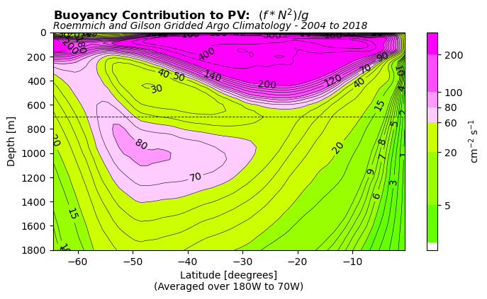
Bouyancy contribution to PV, temperatude and salinity from obs
[35]:
catalog = intake.open_catalog(diag_config_yml['oce_cat'])
ds_obs = catalog['rg-argo-2018'].to_dask()
[36]:
plot_aaiw_pv_obs(ds_obs, levels, colors)
Volume of water with PV > 60 cm-2 s-1: 15.2133647204352 x 1.0e^15